


Taxation and Economic Growth
What the Empirical Literature Tells Us About the Growth Risks of a $4.5 Trillion Tax Hike


Failure to renew the expiring Tax Cuts and Jobs Act (TCJA) of 2017, while unlikely, would constitute a $4.5 trillion tax hike on the U.S. economy over the next decade, with roughly $500 billion of that burden due in 2026 alone. With this risk looming on the near horizon, it might be worth revisiting the empirical literature on the tax multiplier.
Economists have defined the multiplier as the ratio of a change in output to a unitary exogenous change in the fiscal balance—whether from government expenditure or tax revenue.
In simple terms, the tax multiplier measures the effect of changes in taxes on the nation’s economic output, or gross domestic product (GDP). A multiplier of -1 means that every $1 increase in the tax burden reduces GDP by an equal amount ($1). A multiplier of -1.5 means that every $1 increase in the tax burden reduces GDP by a larger amount ($1.50).
Tax multipliers can vary widely based on time horizons and behavioral adjustments. As Valerie Ramey notes in her 2019 study: “Many estimates of tax multipliers start out low on impact but then build.” For this reason, it is helpful to break down multipliers by different time horizons and to review both impact multipliers and peak multipliers. Impact multipliers reveal the near-term (within a few quarters) change in output in response to a tax increase, while peak multipliers represent the maximum change in output over a longer period (typically two or three years). As Ramey alludes, peak multipliers are larger. This is because it takes time for households and firms to fully react to tax changes that amplify the effects over time.
A Review of Empirical Literature
Researchers have used various approaches, from time-series statistical models to narrative historical analyses, to estimate how changes in taxes affect GDP. Estimates of the tax multiplier have varied widely, ranging roughly from -0.5 to -5 depending on the method and context. This section reviews these studies in turn.
One of the earliest studies measuring the impact of taxation on GDP is by Blanchard and Perotti (2002). Using a mixed structural vector autoregression (SVAR)/event study approach, they find an impact multiplier of -0.7 and a peak multiplier of -1.33 for U.S. data over the period 1947 to 1997. Revisiting the issue of the growth impact of taxation, Perotti (2005) applies a vector autoregression (VAR) approach to a panel of five countries in the Organisation for Economic Co-operation and Development (OECD) during the period from 1961 to 2001. For post-1980 U.S. data, the study finds an impact multiplier of -0.43 and a long-run effect of -2.11.
Using an extended sign-restricted SVAR approach, Mountford and Uhlig (2009) find an impact multiplier of -0.28 and a peak multiplier of -3.57 in U.S. data for the years 1955 to 2000. When estimating the present value peak multiplier, they find a more significant impact of -4.98. Meanwhile, Uhlig (2010) uses a dynamic stochastic general equilibrium (DSGE) model (based on the Trabandt–Uhlig model) to derive a long-run tax multiplier of -2.4.
Romer and Romer (2010) apply the narrative approach—identifying exogenous tax changes by using historical records and policy documents to distinguish tax reforms motivated by long-run goals. Using U.S. data for the years 1947 to 2007, the authors find an impact multiplier around -1.2 and a peak multiplier around -3.
Calculating the impact multiplier using a neoclassical model (Barro–King Framework), Barro and Redlick (2011) find a tax multiplier of -1.06. Ramey (2019) notes that this smaller estimate might be the result of Barro and Redlick’s use of various approximations and constraints on dynamics.
Observing U.S. data for the years 1945 to 2009, Perotti (2012) uses a VAR approach to estimate the peak tax multiplier. The author finds a peak multiplier of around -1.7 and one around -1.5 after three years. Finding results within a similar range, Chahrour et al. (2012) apply a DSGE model to arrive at a peak multiplier estimate of around -1.8.
Applying the Romer–Romer narrative approach to United Kingdom (U.K.) data for the years 1947 to 2009, Cloyne (2013) finds an impact multiplier of -0.6 and a long-run multiplier of -2.46. Using the same approach for a sample of 17 OECD countries, Guajardo et al. (2014) find a larger impact on GDP of about -3.1 at the two-year horizon. While applying this approach to data for Germany during the period 1974 to 2010, Hayo and Uhl (2014) find an impact multiplier around -1 and a peak multiplier of -2.4.
Measuring whether the size of tax multipliers is dependent on different states of the economy, Jones and Olson (2014) apply Hansen’s threshold model (1997) to determine the effect of monetary policy on the size of tax multipliers. Using U.S. data for the years 1950 to 2007, Jones and Olson find a peak multiplier of -1.2 under a tight monetary regime and -4.3 under a loose (accommodative) monetary regime. Using a dataset similar to that of Jones and Olson, Mertens and Ravn (2014) adopt an SVAR approach with Romer–Romer shocks and find an impact multiplier of -1 and peak multiplier of -3.
Pereira and Wemans (2015) use the narrative approach to estimate the tax multiplier in Portugal for the years 1996 to 2012. The authors find a large-impact multiplier of -1.8 and a long-run multiplier of -2.8 at the three-year horizon. Using the narrative approach for a sample of advanced economies, Jalil (2016) finds an impact multiplier of -1.22 and peak multiplier of -3.89, while Riera-Crichton et al. (2016) find multipliers of -0.66 and -3.56, respectively.
Measuring the effect of taxation on output for a panel of 16 OECD countries, Alesina et al. (2018) find a peak multiplier of -1.5 using static surplus and -3.7 using the actual response of surplus. Adopting the Blanchard–Perotti VAR method, Afonso and Leal (2019) find a tax multiplier of -1.75 at the one-year horizon for Eurozone countries during a recessionary period.
Applying the narrative approach to a sample of 51 countries over the period 1970 to 2014, Gunter et al. (2021) estimate impact and peak multipliers of -1.1 and -2.7, respectively. When narrowing the scope of countries to only advanced economies, the authors find the peak multiplier to be significantly larger, at -3.6. They find that countries with higher initial tax burdens (typically European Union, or EU, countries) tend to have more negative output effects than those with lower initial tax burdens.
Estimating the growth response to tax shocks using the local projections method of Jorda (2005) with an instrumental variables estimator, Dabla-Norris and Lima (2023) find an impact multiplier of -1.26 and peak multiplier of -2.12 for 10 OECD countries during the period 1978 to 2014. Applying the same technique for a large sample of 177 countries from 1995 to 2019, Geli and Moura (2023) find impact and long-term multipliers of -1.71 and -2.47, respectively.
Observing the effects of personal income taxes on output, Schoder (2023) adopts a DSGE and local projections method for a panel of 75 countries over the years 1994 to 2018. The author finds an impact multiplier of -1.4 and peak multiplier of -2.3 at the three-year horizon. Finally, Kopecky et al. (2024) replicate the approach of Cloyne (2013), using robustness tests to determine the accuracy of Cloyne’s results for U.K. data. The authors find results in-line with Cloyne's estimates, finding an impact multiplier around -0.6 and peak multiplier of -2.23.
Synthesizing the Estimates
Most of the impact multiplier estimates lie between -0.5 and -2, while most peak multiplier estimates fall within an even broader range of about -1 to -3.5. Narrowing down the estimates cited in the literature, the mean value of estimates for the impact multiplier is -1.01, while the mean value of the peak multiplier is significantly larger at -2.33. These figures reflect the raw unweighted averages from the empirical literature. To account for potential outliers or publication bias, I drop the most extreme (~10%) estimates to simulate the Duval and Tweedie trim-and-fill method. The resulting adjusted mean estimates are -0.94 and -2.35, respectively, indicating robustness of the central tendency to outliers.
Taking this a step further, I can narrow down the central tendency of multiplier estimates based on the precision of estimates using a meta-analysis approach. I use two statistical techniques for meta-analysis: the DerSimonian–Laird method (a traditional random-effects approach) and a modern REML (restricted maximum likelihood) approach to account for differences across studies (heterogeneity) while computing an average effect. In essence, both methods weigh the studies’ estimates and provide a combined tax multiplier, with a confidence interval. I start by using a Random Effects (RE) model (DerSimonian–Laird estimator). Table 1 below shows the results from the random effects model.1
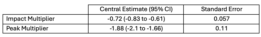
The meta-analysis results suggest that impact multipliers tend to be about three quarters as large as the initial tax shock, while peak multipliers are almost twice as large (~-1.9) as the initial tax shock. However, given the number of studies in this analysis, the variance in standard errors, and the likely true heterogeneity in effects, the DerSimonian–Laird estimator might not be the most suitable method.
The REML method provides better estimates of between-study variance, offers more accurate confidence intervals, and tends to be preferred in rigorous empirical studies. For this reason, I re-run the meta-analysis using the REML method. Table 2 below shows the results from this preferred method (REML).
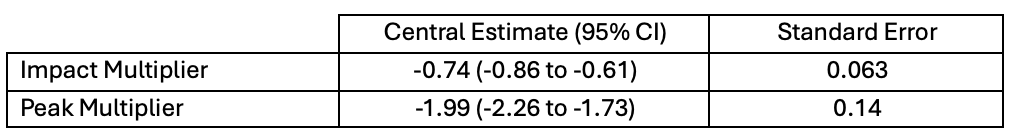
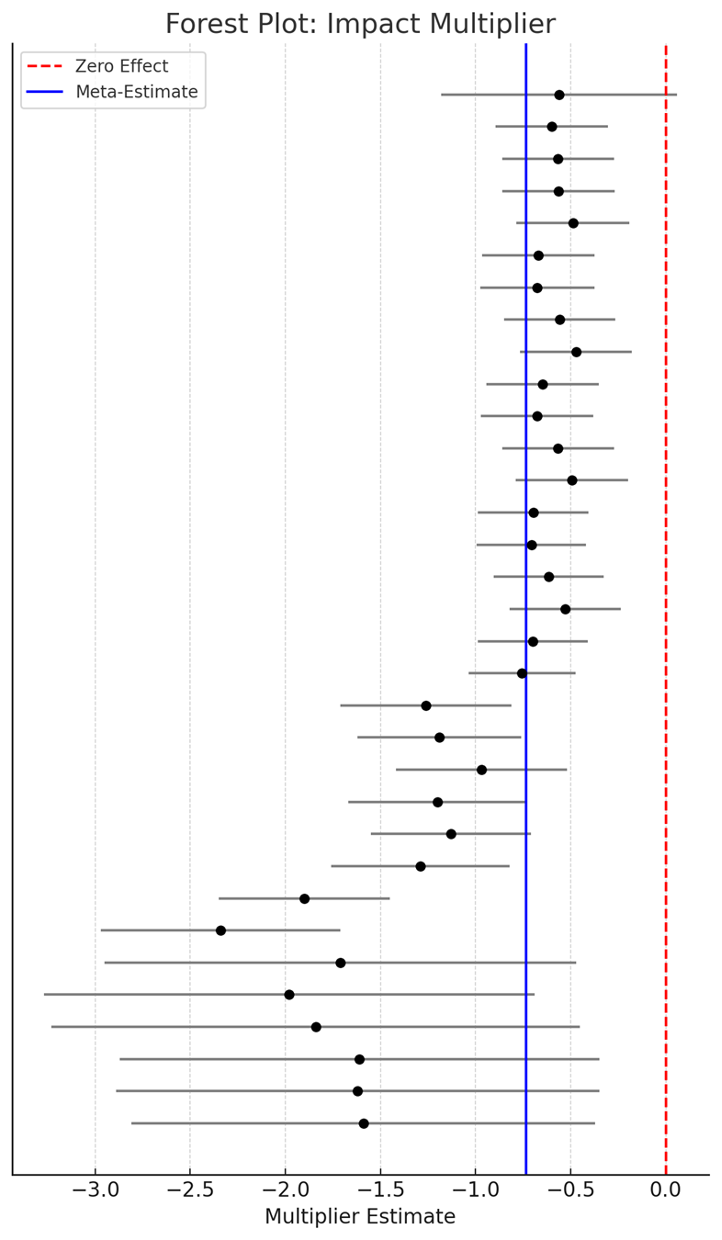
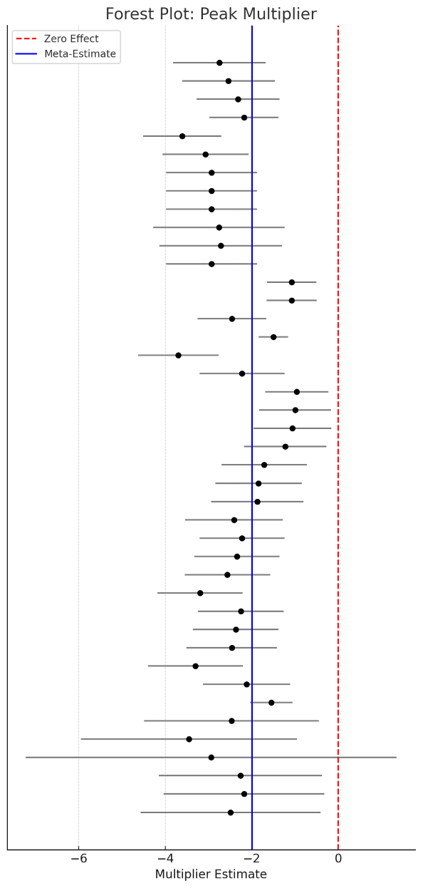
Consistent with the RE estimator, impact multipliers are found to be about three quarters as large as the initial tax shock. However, peak multipliers are slightly larger using the REML method, with negative output effects being twice as large as the initial tax shock. Figures 1 and 2 show the forest plot of study estimates for impact and peak multipliers, respectively.
In sum, most empirical literature suggest that tax increases are associated with a significant, negative, and persistent impact on economic growth. My preferred estimates suggest that in the short term, output falls by about 75 cents for every $1 increase in tax, while the full economic impact is likely to be around $2 for every $1 in additional taxation. Failure to renew the expiring TCJA provisions would amount to a multi-trillion-dollar tax increase that would meaningfully suppress economic growth over time.
In fiscal consolidation efforts, policymakers should prioritize spending restraint to avoid long-term damage to economic growth. When it comes to raising revenues, policymakers should prioritize eliminating and restricting inefficient tax expenditures (deductions, exemptions, credits, exclusions, etc.) that distort economic behavior, misallocate resources, and lead to inefficient outcomes. In a recent paper, my coauthor and I provide a roadmap for achieving a more efficient, more just, and less distortionary tax code, while also identifying low-hanging fruit for policymakers in implementing tax cuts and full expensing without blowing up the long-term budget deficit.
The meta-analysis includes 76 estimates from the empirical literature weighed by precision using standard errors.